Guillermo Angeris, Alex Evans, Tarun Chitra
In the first post of this series, we looked at how the curvature of the trading function of a constant function market maker (CFMM) influenced trader behavior. We illustrated a result from our upcoming paper, ““When does the tail wag the dog? Curvature and market making” that relates price stability to curvature. Recall that informally, the curvature of a CFMM’s trading function describes the absolute change in the price reported by a CFMM after a small trade. When a CFMM is a primary market, the impact that a trade has on secondary markets with the same assets is dependent on the ratio of curvatures of the two markets. This illustrates the idea that price stability between markets is intimately connected to their curvature. But a natural question to ask is: why do rational liquidity providers (LPs) choose to place liquidity on either the primary or secondary markets? And more specifically, how do they measure and/or compare their returns on these markets?
In this post, we will focus on answering these questions from two lenses:
- Formalizing the intuition that LPs make the most money on mean-reverting asset pairs
- Measuring the adverse selection that LPs face when traders have information
The latter view on LP returns is similar to classical market microstructure results from Albert Kyle, Lawrence Glosten, and Paul Milgrom (2020 Nobel Memorial Prize winner). We will show that both of these facets of LP returns are closely tied to curvature. These results show that the shape of a CFMM not only dictates stability as a primary market, but also controls expected LP profit and losses.
Mean-Reversion is Best
For a given price move, a lower-curvature CFMM will engender greater losses for LPs. At the same time, lower curvature provides lower slippage, attracting more traders and fee revenue. Studying the trade-off between impermanent loss and fees allows LPs to optimize their returns. The optimal curvature will depend on the behavior of the market. Here, there are two models we can choose from: One involves modeling an external price process independent of market mechanics, while the other requires directly modeling the microstructure of the underlying market.
In the case of the former, the relevant features of the process are correlation, volatility, and mean reversion. For mean-reverting assets, the return-optimal curvature is usually lower. CFMMs LPs profit from mean reversion as reserves are restored to previous levels while fees are accrued in both directions. In the case of strongly mean-reverting assets, the risk of impermanent loss is therefore lower and LPs can afford to offer lower curvature to attract traders. The most well-known example of this is Curve. Stablecoins generally hover around the price of $1 and deviations from those levels are quickly corrected by arbitrageurs. As a result, Curve offers an ultra-low curvature CFMM, which attracts significantly more trading interest than an equivalent high-curvature pool such as Uniswap would for those pairs. As long as stablecoins continue to revert to the mean of dollar-parity, Curve LPs will outperform LPs in higher-curvature CFMMs. A number of protocols have trading functions that change as a function of time. Below, we see the marginal price functions for Yield (left) and Notional (right).
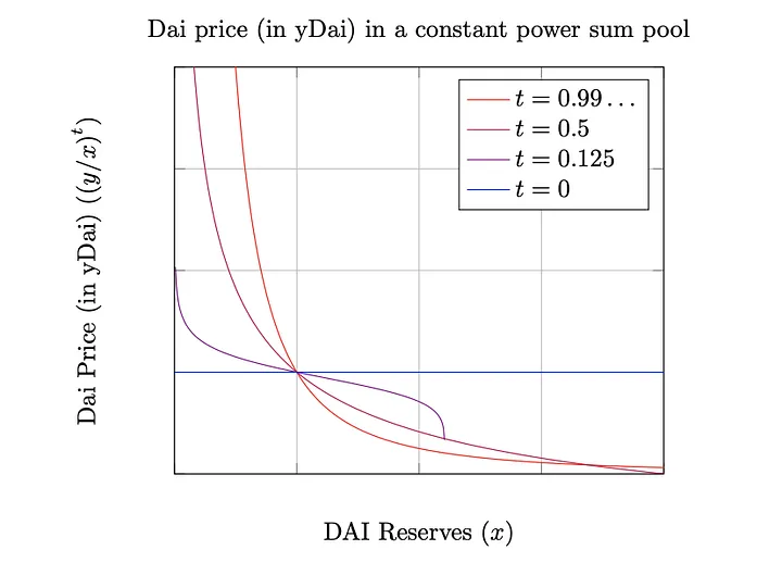
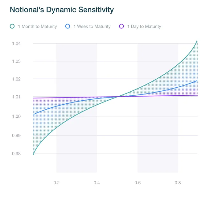
Both of these protocols aim to provide fixed-interest loans and effectively utilize the curvature of the CFMM to control the incentives of users. At time t, users of these systems effectively create a fixed interest rate, zero-coupon bond that matures at time t+T. When a user creates a bond, they mint it at a price less than 1 bond / 1 Dai. A user can trade their bond in the CFMM market for Dai and the slippage they face reflects a cost of early redemption. This is analogous to early redemption of bonds in the traditional repurchase agreement market. As we approach time t+T, the CFMM curvature goes down, incentivizing users to close their bond out (e.g. trade it for Dai). At expiry, the CFMM has no curvature, which means the user can redeem their bond 1:1 for Dai. Note that the design of these CFMMs encourages mean-reversion (e.g. to 1:1) as we get closer to expiry. Our results above suggest that when designing such mechanisms, one needs to also adjust the fees to ensure that LPs are profitable.
Market Microstructure
Another way to describe LP returns is to consider the expected profits in a game between the LP, an arbitrageur, and an informed trader. To construct our game, we first draw inspiration from the traditional market microstructure literature. Tomes from this literature, such as Kyle’s Continuous Auctions and Insider Trading (1985), consider games between market makers (who stay delta neutral) and noise and informed traders. In these models, it is assumed that each participant has a strategy that provides a price and quantity that they are willing to trade on. For instance, the informed trader might know that the earnings per share of an asset is going up and aggressively buys until the new price to earnings ratio is the same as the original. On the other hand, a market maker has a strategy for producing a price and quantity that they are willing to quote within an order book, whereas a noise trader purchases a completely random quantity. Given the set of market participant strategies, we then seek to find out if there is a market equilibrium and if so, if we can compute it.
In general, it is quite difficult to compute exact equilibria in multiplayer games for both computational complexity and statistical reasons (c.f. a previous post from Gauntlet). However, by studying a simplified game, we can garner enough intuition to design a numerical simulation that can estimate a realistic equilibrium. This is precisely what Kyle (1985) and Glosten and Milgrom (1984) do by considering a game with only three players.
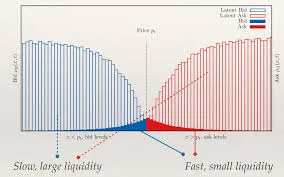
In these games, equilibria are usually found by enforcing a zero-profit condition on market makers (a weak form of no-arbitrage). The zero-profit condition effectively represents a ‘break even’ point for the market maker and is a function of the fees charged and the informational advantage of the informed trader. For instance, if the informed trader has a weak informational advantage, then their trades look like ‘noise’ and market makers make money as the bid/ask spread is crossed repeatedly and the price looks weakly mean-reverting. On the other hand, if the informed trader is omniscient and always knows the future price moves ahead of time, then the market makers need larger fees and a wider bid/ask spread to compensate for trades moving against them. In such a scenario, we say that the market maker undergoes adverse selection from the informed trader. Effectively, market makers respond to an increase in adverse selection by making a market less liquid. Glosten (1994) showed that when you consider market makers who have to quote prices on multiple markets, then the shape of the order book impacts how liquidity changes in response to adverse selection. In the image below, we see two different shapes for an order book, one approximately concave (the unshaded bars) and one convex (the filled in region). Glosten showed that the concave shape is better for large liquidity and low trading velocity (e.g. trades per second) whereas the convex shape is better for many small orders and high trading velocity.
Recent work by Jun Aoyogi of Berkeley, shows that results similar to Kyle (1985) can be found for Uniswap by considering a simple one-period game between an LP and an informed trader. In particular, he shows that LPs can only make money if noise traders trade against Uniswap and if the fees correctly compensate for volatility caused by noise traders. Moreover, he also illustrates a price stability result (akin to what we covered in our first post). However, these results rely quite heavily on the simple functional form of Uniswap’s constant product formula. Moreover, precise bounds on the amount of fees needed to compensate for adverse selection is not covered in these results. Can we relate fees and adverse selection in a more general way for other CFMMs?
To do this, we construct a different game between arbitrageurs, informed traders, and LPs. We first define an informed trader as a participant who has at time t, a probability 𝛼 > ½ of knowing the price of the asset at time t+1, p(t+1). We write the informed trader’s prediction of p(t+1) as p_inf(t). We can think of this as the informed trader flipping a coin that has probability 𝛼 of landing on heads and 1-𝛼 of landing on tails. If it lands on heads, the trader correctly picks the next price. This clairvoyant participant trades with the CFMM at time t and realizes a profit at time t+1 with probability 𝛼. On the other hand, if the informed trader loses, the price reverts to its value at time t. Schematically, this looks like the following:
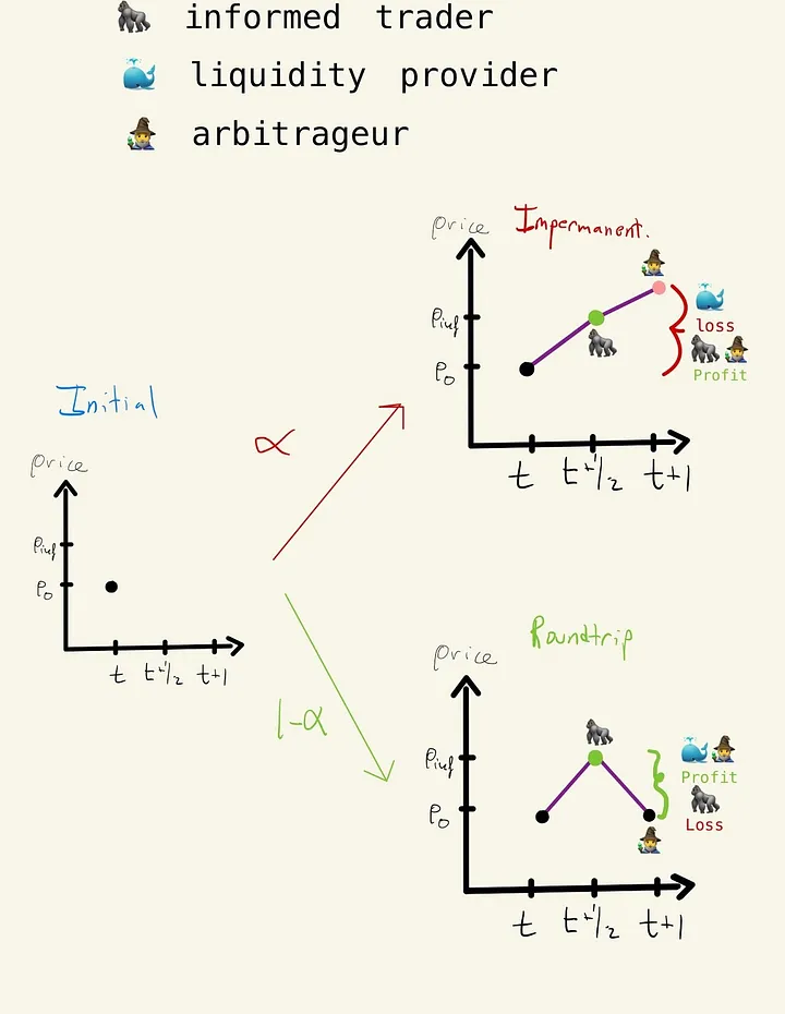
Note that when the informed trader loses, the price goes from p(t) to p_inf(t) back to p(t). In this ‘roundtrip’ sequence of trades, the profit earned by the liquidity provider is a function of the fees and the curvature of the CFMM. In particular, we show that the expected loss of the LP is at least:

Where κ is a parameter that captures curvature and γ is one minus the fee percentage. Here, the surprising fact that the fee γ appears in the denominator (versus, as one might expect, in the numerator) happens because the final price depends implicitly on the fee charged. Note that, if κ is very small (ie, the CFMM has low curvature) then the minimum loss is large; similarly, given two CFMMs, one with lower and one with higher curvature, α, the edge, needs to be larger in the CFMM with higher curvature to achieve the same lower bound for the loss.
In the figure below, we see schematics of how such protocols adjust the curvature of their trading function in response to trading activity. This effectively reduces the adverse selection by increasing curvature in response to an informed trade. Currently, most curvature adjustments are exogenous, requiring an outside oracle to trigger a curve change.
Moreover, this also tells us that markets that are active and have low curvature CFMMs, such as Curve, tend to have less informed trading. This matches the intuition that traders who swap one stablecoin for another have less useful information about the future price, but are rather going from one stablecoin to another to optimize yields or move between different centralized exchanges.
Future CFMM design
What does this tell us about how to design CFMMs? Firstly, the somewhat ad hoc usage of oracles to correct curvature can be improved by designing the CFMM’s trading function in a manner that meets the informational advantage of traders vs. LPs. A market maker could have a dynamically updating trading function that reacts to trades to reduce LP impermanent loss. The update rule could be purely endogenous (unlike designs using oracles) and a simple control mechanism (akin to a DeFi PID controller; see the previous post from Gauntlet on this topic). Similarly, a gradient flow for a CFMM’s curvature (e.g. akin to the famous Ricci flow) could be used to naturally flatten regions with low trading volume due to high slippage. Designing such CFMMs cannot be done analytically, unfortunately. A practical CFMM of this form needs to be designed by simulating multiple agents with differing amounts of information and strategies interacting with liquidity providers. Moreover, if we see the sophistication often found in high-frequency trading, we should expect that dynamic LP strategies will become the norm in the future. The effect of these strategies on curvature and adverse selection would also need to be modeled by agent-based modeling.
We want to thank James Prestwich and Ciamac Moallemi for helpful comments and suggestions
Blog
View the full presentation
Read the full paper


