Summary
Gauntlet has executed 13 proposals during the most recent Compound engagement, the first of which was executed on 11/09/2021, the last of which was executed on 07/04/2022. Gauntlet increased Collateral Factors (CFs) in every proposal, except for one time decreasing the CFs of BAT and ZRX on 11/27/2021, which were later increased.
Below is the time series of collateral factors for each asset from 11/01/2021 (8 days before the engagement), until 08/15/2022.
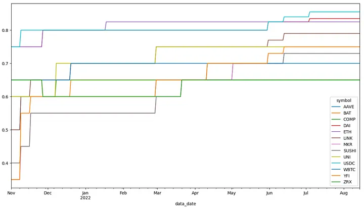
The resulting proposals resulted in net CF increases for the majority of assets, all while incurring no insolvencies despite significant market volatility, as outlined in our Market Downturn Analysis posts. In each of our forum post proposals we include screenshots of the projected increase in VaR and LaR (proxies for risk) as shown below.
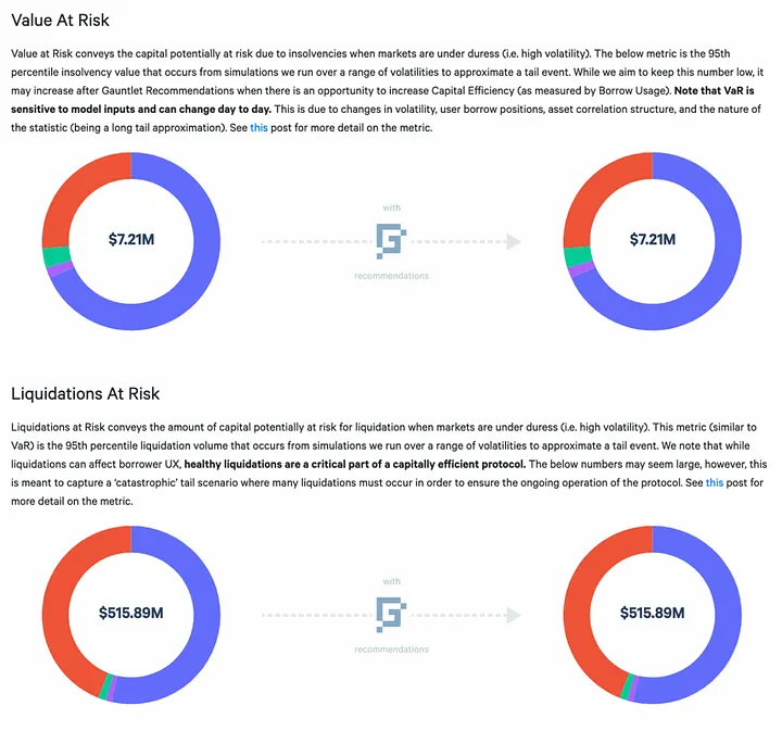
Since we do not expect our recommendations to increase protocol risk, these collateral factor changes proceeding without insolvency was a successful result for our product. But what value did Gauntlet add to the protocol as a result of this? Besides managing risk, we seek to confirm that our recommendations generated quantifiable increases in usage and revenue, which will be the main topic of this case study. Using the methodology detailed below, we found that Gauntlet’s impact totaled $96M in added borrows and $5.15M in added borrow interest over the course of our engagement with Compound.
Expected Impact
When collateral factors increase, we project users to take advantage of some of their additional borrowing power. Thus, we can think of expected impact as the increased usage that we estimated at the time the change was made. As changes go live, we can then calculate how much of this additional usage is realized, which depends on market conditions and user behavior. To make this more concrete, let’s review the formal definition of borrow usage, which we introduced previously here,
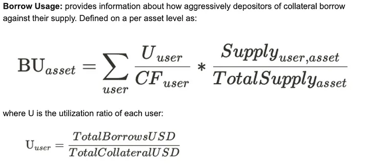
Essentially, for a given asset, the borrow usage is the average percentage of borrowing power used by each user of the asset, weighted by their share of total supply in that asset. The system borrow usage is the average of each symbol’s borrow usage, weighted by the protocol percentage supply. It can be a little hard to intuit however, so let’s take a look at an example.
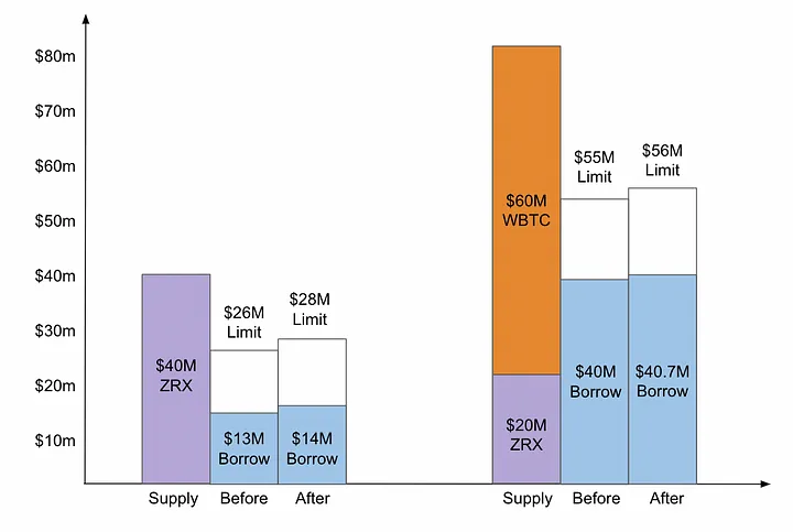
Imagine the total supply of ZRX in Compound is $60M, and it is composed of two users who supply $40M and $20M ZRX, respectively. The current CF of ZRX is 65%, and we want to know what the increase in borrow usage will be if we increase the CF to 70%.
Taking a look at the first user, we see he has supplied $40M ZRX and no other assets. As a result, this user has $40M * 65% = $26M borrowing power, and has decided to borrow $13M USDC, so this user’s initial borrow usage was $13M / $26M = 50%. With a CF of 70%, the user now has $40M * 70% = $28M borrowing power. In order to keep the borrow usage consistent, this user will borrow $28M * 50% = $14M USDC. As a result of the change, we would see a $1M / $13M = 7.7% increase in total borrows and borrow usage.
The second user has $20M ZRX supplied, but also $60M WBTC supplied. WBTC has a CF of 70%. As a result, this user has $20M * 65% + $40M * 70% = $55M borrowing power, and has decided to borrow $40M USDC, so this user’s initial borrow usage was $40M/$55M = 72.73%. With a ZRX CF of 70%, the user now has $20M * 70% + $40M * 70% = $56M borrowing power. Note that the increase in borrowing power is relatively smaller compared to the entire supply position, because ZRX only makes up 25% of the supply for this user. In order to keep the borrow usage consistent, this user will borrow $56M * 72.73% = $40.73M USDC. Proceeding similarly for this user, we would see a $0.73M / $40M = 1.8% increase in total borrows and borrow usage.
Essentially, we see that the increase in borrows for each user is the ratio of the old and new collateral factors (70% / 65% ) -1 = 7.7%, multiplied by the percentage of the user’s supply which is ZRX. So if the suppliers of a given symbol have even more supplies of other assets, we do not expect to see large borrow usage changes as a result of that symbol.
The assumption that borrowers will increase their borrows to take full advantage of their increased borrowing power as a result of our parameter recommendations is what we refer to as elasticity, which we will assess later. However, assuming that users are indeed elastic, we can obtain our projected borrow usage increases and an impact dollar value.
Impact Metrics: Borrow vs Interest
Referencing the Borrow Usage visual above again, if we were to increase the CF of ZRX, we see that there is a projected dollar increase in total borrows for each of the users that supply ZRX. Given that about 94% of all borrows in Compound are stablecoins, this usually results in an increase in stablecoin borrows. However, we may care more about the increase in borrow interest of these borrowed assets, since that’s extra income the protocol can decide to either allocate to suppliers (to incentivize more TVL) or to the reserves (to be able to cover insolvencies or other unexpected events). Therefore, we will include the projected increase in borrows in our numbers, but use projected increase in interest as the primary metric for Gauntlet’s impact.
The way to calculate the annual projected increase in borrows for a given CF change is to iterate over every user that supplies assets, calculate the projected dollar increase in borrows for that user, and multiply that increase in borrows by the borrow rate for each borrowed asset. So if a CF increase in ETH results in $25M projected increase in USDC borrows relative to the previous CF, and the borrow rate for USDC is 4%, this would result in a projected USDC-specific annual impact of $25M * 4% = $1M. Note that in reality an increase in USDC borrows would increase the USDC utilization, thus increasing the borrow interest and even more projected impact, but for simplicity we can assume the borrow interest is static.
Gauntlet’s projected annualized increase in borrow interest at the time of our CF changes was $24M total. However, projected annualized impact assumes that total borrow amount and borrow rates remain constant throughout the year, which of course will not happen. Even though our projected impact was $24M, we may actually see more or less depending on realized market conditions. Since we simulate a range of outcomes and do not attempt to predict the overall direction of markets, our pre-recommendation estimates assume market prices and interest rates remain unchanged throughout the impact period.
Calculating Realized Impact
To calculate our realized impact, we must:
- Account for the fact that realized borrows and borrow rates change over time
- Verify our elasticity assumptions
Incorporating the realized borrows and borrow rates is relatively straightforward to do, given we have daily borrower data and can calculate interest from the known borrow rate on that day. Verifying the elasticity assumption is more complex. To better illustrate, let’s look at the following example:
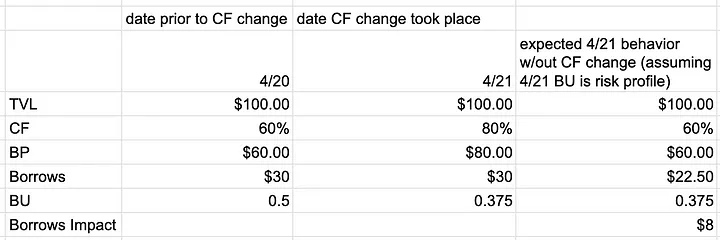
Imagine there is a user who on 4/20 supplies $100 of DAI, which has a CF of 60%, and borrows $30 of DAI. Assume DAI CF increases from 60% to 80% on 4/21, but the user’s TVL and borrows remains the same. Now we’re left with the question of, “what was our realized impact of this user on this date?” There are a couple ways we could think about this.
Constant Usage View
We could see this case as showing zero realized impact, since the user did not increase their borrows to take advantage of their increased borrowing power. Essentially, assuming that the user’s risk profile was established on 4/20, this user was not elastic. It is tough, however, to compute long term impact in this framework, since users’ risk profiles change, and it is not always clear which changes in borrow usage are due to updated risk profiles as opposed to elasticity. As we will later discuss, this assumption is appropriate for some users, but in general we use a more flexible elasticity assumption described below.
Dynamic Usage View
We could also say the user understood that they had increased borrowing power on 4/21 and changed their risk profile purposely such that their new comfortable borrow usage was 37.5% (due to market volatility or whatever other reasons). We can then posit that if the DAI CF hadn’t increased, the user actually would have decreased their borrows to maintain their new baseline 37.5% borrow usage risk profile.
This framework allows us to more cleanly calculate impact, since we can update the user’s risk profile with each data point as we get more info on their behavior. This avoids the issue of having to choose a time in the past to use as the benchmark for risk tolerance, which is a problem for volatile assets. Of course, we still have to make sure usage is stable in the long run to validate elasticity, but this is much more realistic than expecting it would be constant on a daily timescale for most users.
Observing User Elasticity
From the real data, it may or may not be possible to identify an appropriate constant risk profile for every user. In our analysis, we use both frameworks described depending on how we classify an account. The two types we use here are:
- Recursive: These are users who have exactly one symbol with a positive supply and borrow. For example, a user who has $1M DAI supplied and $500k DAI borrowed is a recursive account. Since recursive users restrict their activity to one symbol, their usage is less sensitive to relative price fluctuations. For these accounts, we found it appropriate to assume constant usage as they are observed to fit this behavior quite accurately.
- Non-Recursive: These are all other users who do not exclusively borrow and supply only one symbol. Though accounts in this group may have some overlapping borrow and supply symbols (i.e. partially recursive users), their exposure is not insulated from market volatility like that of a purely recursive user. We thus consider it more appropriate to apply the dynamic usage framework for this entire group of accounts.
Performing the calculations for every user and every date during the most recent engagement starting 11/9/2021 until 08/15/2022, we found that the realized interest impact given the above reasoning is $5.15M. Now let’s go forth and analyze the elasticity assumption.
The realized impact we observed is broken down by borrower type as follows:
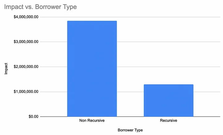
In the above chart, the inner pie sections correspond to the user impact density. For example, in the Non Recursive section, the blue inner pie piece corresponds to the impact came from the largest impact Non Recursive user, the orange piece corresponds to the impact from the second largest impact user, etc., and the brown piece at the bottom aggregates the impact across the remainder of users. Let’s zoom in on the impact of the largest individual borrowers, during which we will determine if our elasticity assumption holds up.
Recursive User Examples
The total impact for recursive borrowers was $1.3M, broken down as follows:
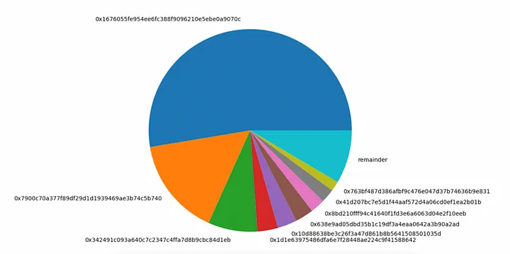
The above pie chart shows that the top 9 accounts account for over 85% of the total recursive impact. Let’s analyze some of the top users descending order of impact to see if the impact is justified.
Recursive User 1
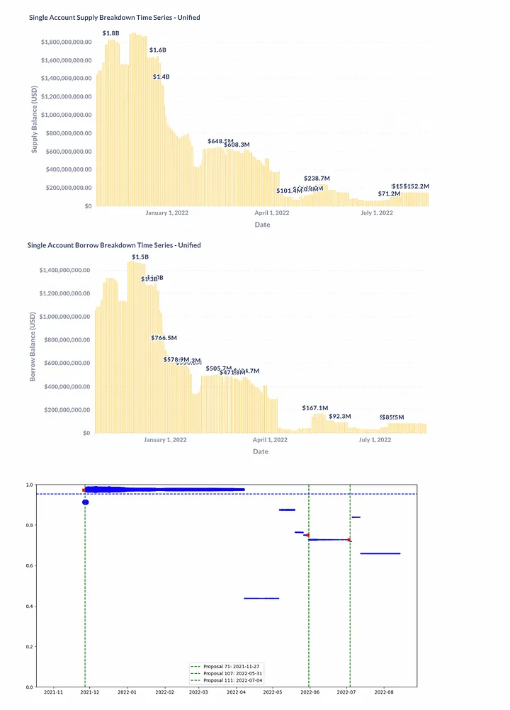
In the above charts we see supply, borrow, and usage time series for the highest impact recursive user, a large USDC account. On 11/27/2021, we increased CFs from 75% to 80%, at which point the user’s borrow usage decreased. However, a few days later, the user updated their position to take full advantage of the increased borrowing power, thus showing the user was elastic. Eventually the user decided to decrease their borrow usage in April 2022 with no collateral factor change. There were 2 more relevant proposals afterwards, when the user had lower TVL. After the second proposal it seemed the user did not update their position to keep their previous borrow usage, but after the third proposal the user increased their borrow usage even higher than it previously was, just to decrease it again later. As we know, it isn’t always clear to distinguish between the user updating their position to be elastic and return to a previous baseline borrow usage, or when a user has determined to move to a new baseline borrow usage. But looking at this user’s behavior, we should be able to at least claim impact through April 2022 based on the constant usage framework, which we do for this account.
Recursive User 2
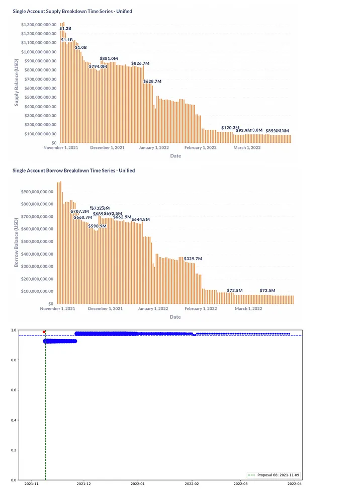
In these charts we show the same data for the next largest recursive account, a recursive DAI borrower. On 11/09/2021, we increased CFs for DAI from 75% to 80%, at which point the user’s borrow usage decreased. However, a few weeks later, the user updated their position to take full advantage of the increased borrowing power, thus showing the user was elastic. Though we could claim impact immediately after the proposal by positing that the user’s risk profile may have also changed, from the chart it seems fairly unlikely that is the case. As a result, for this user we will take the baseline borrow usage to be what it was the date prior to the first proposal, and only claim impact with the constant usage framework described above.
Non-Recursive User Examples
Moving on to non-recursive borrowers where our impact assuming elasticity was $3.85M, the pie chart shows that the top 9 accounts make up about 50% of the total impact here.
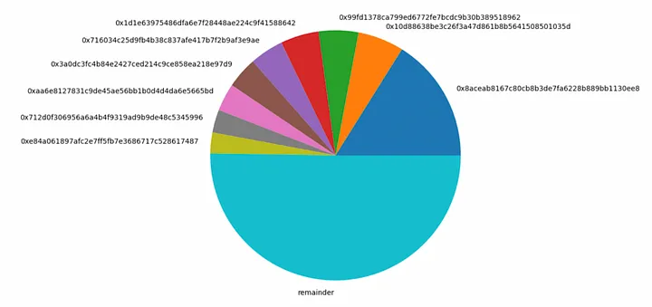
Let’s again look at some the largest users to see if the impact is justified.
Non-Recursive User 1
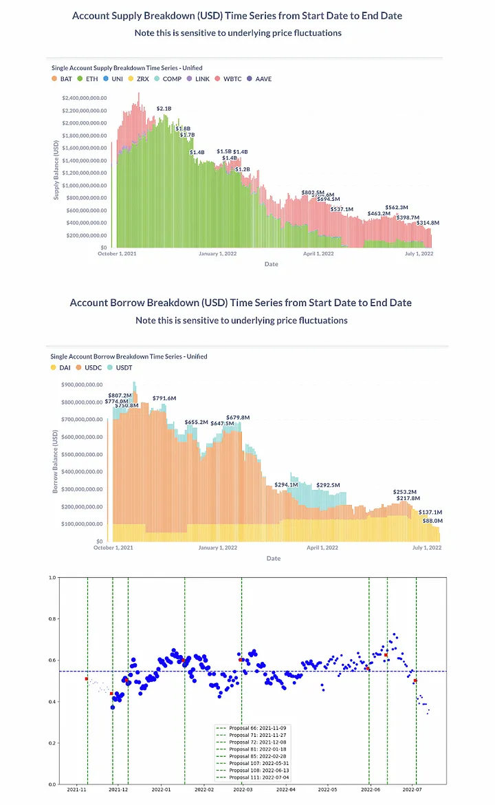
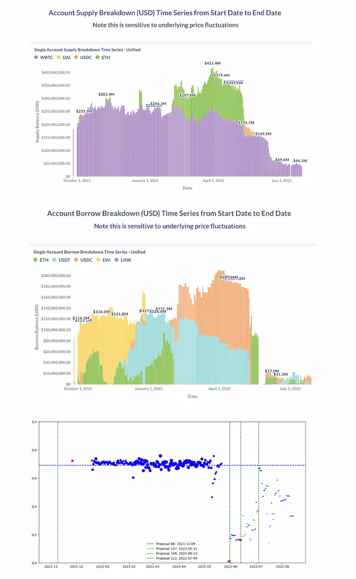
The above charts shows the largest non-recursive user’s borrow usage over time. Dots are weighted by how much impact they drove on that particular day. The vertical green lines indicate the dates of relevant proposal changes for this user (where CFs of symbols this user supplied were increased). The red dots indicate user’s borrow usage on the date prior to the proposal change. The blue horizontal line is the weighted borrow usage across all dates. As we can see, the user tends to hover around a borrow usage in the mid-50% range throughout the course of their interaction with the protocol, sometimes letting their borrow usage increase to roughly 70%, and decrease to roughly 40%. There doesn’t seem to be any clear pattern of decreased borrow usage over time, which justifies this user as elastic. The results for other non-recursive users are very similar, with some more examples shown below. As a result, we will claim $3.85M as realized impact for non-recursive borrowers under the dynamic usage framework.
Non-Recursive User 2
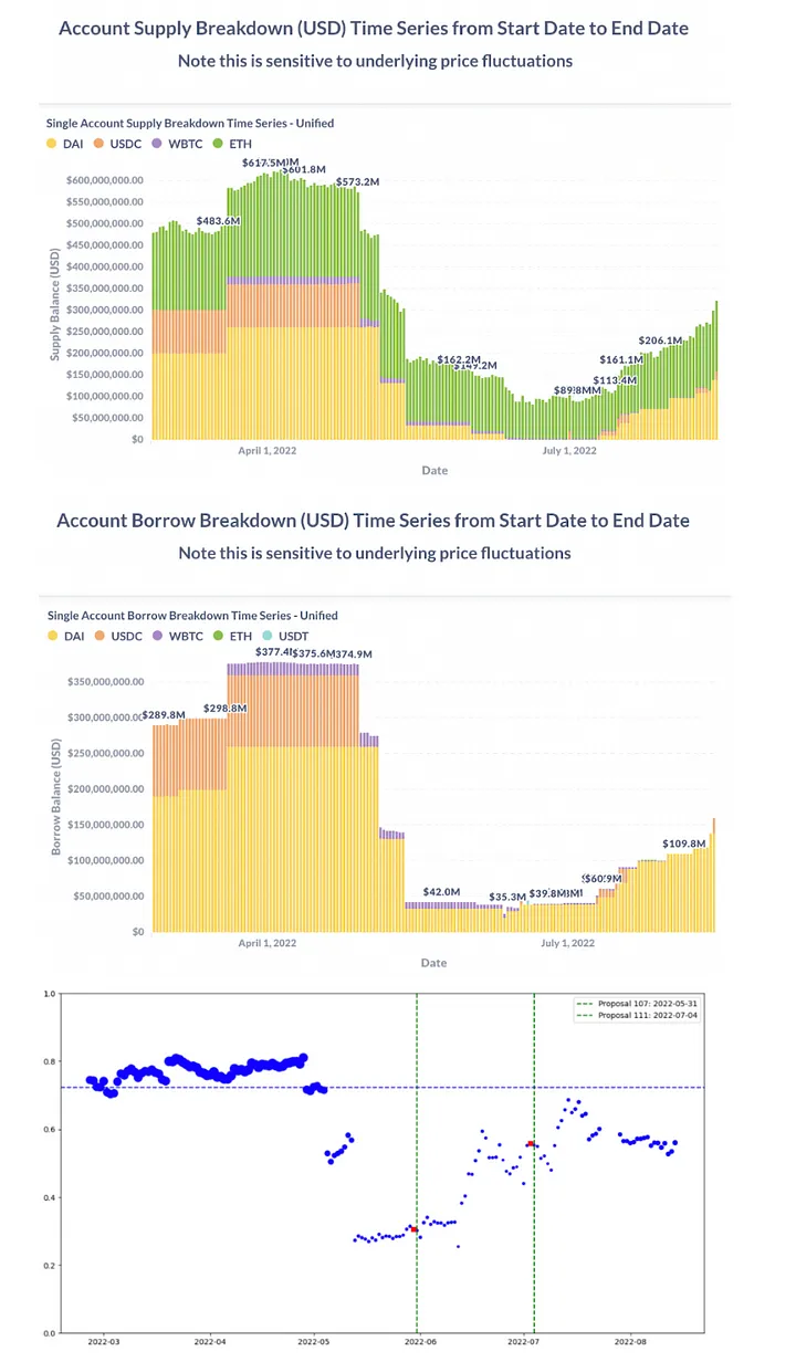
Non-Recursive User 3
Additional Impact on TVL and Future Interest
Another important concept we haven’t touched on — because of how difficult it is to quantify — is how many new borrowers joined Compound as a result of our capital efficiency improvements, how many borrowers decided not to leave Compound as a result of our capital efficiency improvements, and how many existing borrowers decided to increase their borrows / decrease their borrows less as a result of our capital efficiency improvements. During the market crashes, and after the proposal which cut COMP rewards, many users did decide to leave the protocol. It’s very likely capital efficiency improvements kept certain users from leaving and seeking better yield elsewhere. As a basic example, let’s look at the TVL time series of SUSHI, over a chart of our CF recommendations.
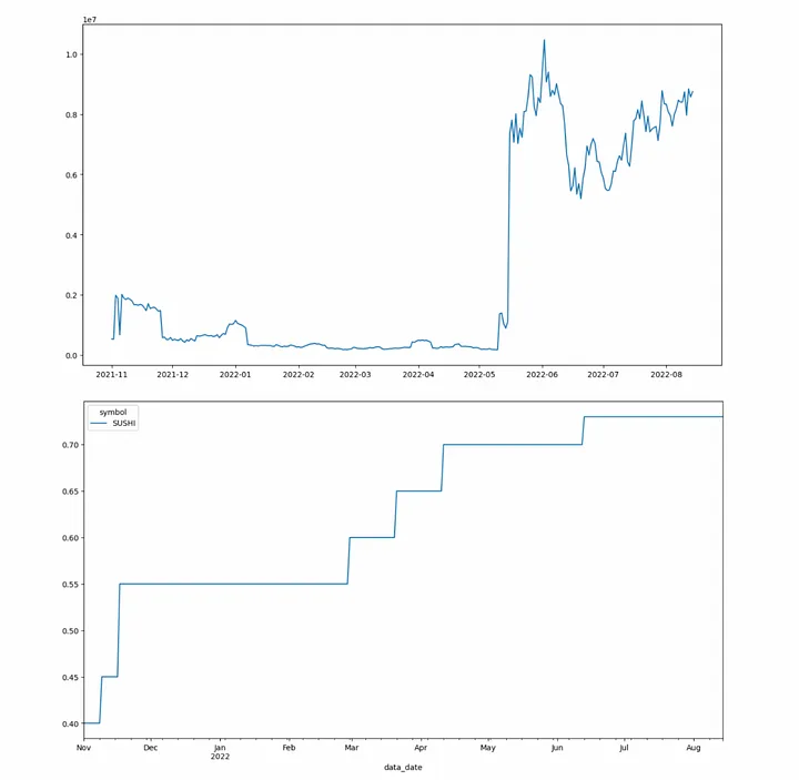
We see that the TVL for SUSHI (due to one SUSHI whale) increased from roughly $0 to $8M shortly after a set of proposals which increased SUSHI CF from 40% in November to 70% in mid April were executed. It’s probably safe to say that this SUSHI whale would not have entered the protocol if not for the drastic increase in capital efficiency. Yet we claim very little SUSHI impact because our calculations assume TVL would be the same regardless of our recommendations. There are similar examples with other symbols that saw TVL rise materially at times, such as MKR, LINK, and AAVE.
Finally, the impact we have claimed so far is only from the realized borrow interest that has already occurred due to our increased CFs. Assuming CFs remain the same, the protocol will continue to benefit from higher interest going forward, which we do not include in this case study. Since these more indirect forms of impact would likely be material, we see the calculation here as a conservative estimate of the most quantifiable value we added. As we refine our methods, we may be able to better measure other types of impact in future case studies.
Case Study
View the full presentation
Read the full paper


.png)


