Guillermo Angeris, Alex Evans, Tarun Chitra
In the first two posts of this series, we introduced the concept of the curvature of a trading function. Curvature gives us a sense of the liquidity of a CFMM: Higher curvature implies higher slippage for a given trade. Today, we’ve published some work that formally describes the results cited in these three posts. First, let’s recap the discussion so far.
In Part I, we showed that observing the ratio of curvatures of two markets gives us a model for stability in CFMM-driven markets. In particular, we discussed the increasingly common scenario when the CFMM is the most liquid venue for trading — i.e. when it has lower curvature than the external market. We showed that this leads the external market to adjust to the price of the CFMM. We also saw that this phenomenon can explain the price-stabilization induced by low-curvature CFMMs like Curve on pegged assets like sUSD. However, we also noted a key limitation of the model: It didn’t account for the effects of external incentives on price stability and curvature.
In Part II, we discussed how curvature affects LPs in the presence of traders with asymmetric information. We saw that the fee required to ensure that LPs remain profitable in the presence of informed traders depends on the curvature of the CFMM. However, in practice, most CFMMs incorporate liquidity incentives in the form of yield farming. There are two natural questions to ask. How should incentives impact the calculation of an LP’s returns? How should protocols efficiently incentivize liquidity?
In the final post of this series, we discuss two approaches to limiting losses associated with curvature. The first involves the LP directly hedging their losses on the external market. Hedging of this form is analogous to that of US equities — traders manually purchase derivative securities like options to hedge risk. The second involves the more recent phenomenon of yield farming wherein protocols incentivize liquidity provision. Yield farming, which is somewhat akin to maker-taker rebates from centralized finance, has driven a lot of the recent growth in CFMMs. Nevertheless, it’s worth asking how much is too much. Over-incentivizing liquidity is not only counter-productive, but can sometimes induce the opposite effects than intended. We sketch a framework for determining a sufficient incentive for liquidity provision.
Hedging as an LP

Recent work by Jun Aoyogi and Martin Tassy, et. al have shown that there are conditions where Uniswap is profitable for LPs, even in the presence of informed traders. This means that despite so-called ‘impermanent loss’, LPs can still end up earning positive returns. By including a curvature correction term, we conjecture that we may be able to expand these Uniswap-specific results to arbitrary CFMMs such as McDEX, Dodo, and Curve. A natural research question, given a framework for bounding impermanent loss for generic CFMMs, is whether it is possible to limit or restrict this loss.
Firstly, we note that it is impossible to completely remove impermanent loss. This is a necessary opportunity cost that must be paid for any derivative asset and is integral to the oracle function of CFMMs. However, just as derivatives portfolios can be used to hedge or reduce such costs, they can also be used to hedge impermanent loss. There have been a number of heuristic approaches — using, for example, options and swaps — that aim to approximately use derivatives to reduce impermanent loss. Many market participants cite this as one of the largest impediments to growing CFMM market share (relative to centralized exchanges).
Given that convexity costs are connected to the curvatures of derivative payoff functions, it is unsurprising that curvature affects the corresponding costs of a CFMM. In fact, much of our work was inspired by the connections between derivative pricing and LP returns described in previous studies. Traditionally, a derivative security is hedged in one of two ways: statically or dynamically. A static hedge takes two distinct portfolios of securities P and Q such that at all times Returns(P) = Returns(Q). If Q is a static hedge for P, Q is said to be a replicating portfolio for P. For instance, the put-call parity formula for options shows that a portfolio P that is long a call and short a put is equivalent to holding a particular combination of the underlying and cash in a portfolio Q. For complicated payoff functions, static hedges will typically require a variety of options, which can be expensive to construct when liquidity is limited.
When faced with practicalities that preclude static hedging, traders often dynamically hedge. The idealized example of this is delta-hedging, where a trader effectively replicates a short position in a derivative by dynamically trading in the underlying to offset any changes in the derivative’s price. More precisely, a portfolio consisting of a single asset S and derivatives on S is delta-hedged if the value of the portfolio doesn’t change when S changes. However, the theoretical delta hedge is never implemented in practice because the requisite liquidity on one side of an order book may not always exist or is too expensive. One famous example of this in quantitative finance is the saw-tooth pattern that has been observed when an investor fails to account for limited liquidity when delta-hedging a position in options.
When there is limited liquidity on the order book, market makers may resort to approximate hedging. In this situation, instead of replicating a portfolio P with a portfolio Q, we instead try to find a portfolio Q such that Property(P) = Property(Q) even if Returns(P) != Returns(Q). In the market maker case, the portfolio Q would consist of L long assets, S short assets, C calls on the asset, and P puts on the asset. For example, a reasonable first approximation for a market maker might be to maintain a market-neutral portfolio — one with zero delta. However, even a small price move can cause a large change in delta, forcing the trader to rebalance to maintain a market-neutral position. When liquidity is limited, such transactions can be costly. Some approximately hedge by neutralizing delta and gamma (the change in the position for an infinitesimal change in price) to minimize the frequency of rebalancing. However, when options markets are less liquid, finding the right combination of derivatives to offset both first and second order impacts of price fluctuations may be too expensive. This puts LPs in a precarious position for all but perhaps a few ETH-USD pools.
So, what can an LP do to cheaply maintain neutrality? We conjecture that a possible answer may be to establish a delta-neutral position, while trying to ensure some bounds on how delta will change as a function of price. For example, for stablecoins, an LP could assume that if prices don’t fluctuate too far from the peg, the absolute value of their delta will remain bounded within some interval. In the paper we show that this bound depends on the ratio of curvature and true market impact for a given trade. More generally, delta will change less after a given price change as the curvature of the CFMM increases. Because hedging CFMMs with illiquid assets can be difficult, CFMMs protocols have often turned to external incentives in order to attract liquidity.
Yield Farming for CFMMs
In our discussion of sUSD in Part I, we noted that the start of yield farming after June 2020 effectively ended the period of price stability that sUSD enjoyed for the prior three months. In a naive model, yield farming should incentivize more liquidity in Curve for sUSD, lowering curvature to engender even greater stability. In fact, the opposite occurred. Part of the reason was that demand for stablecoins during this period was extremely high. Depositing sUSD in a CFMM could result in astronomical “APYs” due to yield farming subsidies. Unlike centralized stablecoins, the creation-redemption process for sUSD and Dai was expensive as it required large amounts of collateral and gas. But collateral was also in short supply during this period, causing stablecoins to break their pegs to meet volatile demand. In other words, over-incentivizing liquidity had the opposite effect of destabilizing stablecoins. But how much liquidity incentive is sufficient?
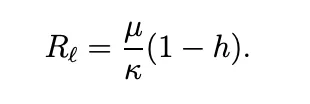
An equivalent question might be to ask: What is a sufficient incentive to entice an LP to provide capital that they would otherwise hold? In the paper, we show that a sufficient per-trade incentive is a simple function of the curvature of the CFMM (μ) and the external market (κ) as well as the expected rate of growth of the asset (h).

In other words, the total quantity of subsidy is proportional to the curvature
of the CFMM and inversely proportional to the curvature of the external market. Typically, a CFMM’s curvature will decline as its TVL increases. In this case, a larger liquidity incentive is required when the CFMM is small relative to the external market.
This result applies to a per-trade incentive when the alternative for an LP is to simply hold the assets. In practice, multiple protocols compete for the LP’s funds. What is a sufficient incentive to entice an LP to switch from one CFMM to another?
The question is particularly relevant to the “vampire attacks” we saw in the summer of 2020. By forking the original codebase and adding a new liquidity incentive, Sushiswap was able to attract significant liquidity away from Uniswap and Swerve challenged Curve. These were otherwise identical to the original CFMMs, except for the governance tokens they issued to incentivize users to switch. To model the difference, consider that the original CFMM starts out c times larger than the challenger (fork). Here we ask the question: what is a sufficient per-trade subsidy to entice the LP to always choose the challenger CFMM? We show this amount to be:

In other words, to successfully execute a vampire attack, it is only necessary for the challenger to incentivize liquidity up to the point where its reserves exceed those of the original. After that point, the fork becomes more attractive to supply liquidity to than the original on its own, requiring no further subsidy. Another way of interpreting the result is, all things being equal, it is preferable to supply liquidity to a CFMM with higher TVL, even in the absence of fees. This has more to do with the fact that a more liquid CFMM is more stable for the LP. We expect the introduction of fees to accentuate this effect further as higher TVL tends to attract disproportionately more trading fee revenue.
Blog
View the full presentation
Read the full paper


.png)


